


Getting Started#
The Acoular library is based on Python. This guide walks through a small frequency-domain beamforming workflow using the same example scripts that are built and tested in the documentation gallery.
Prerequisites#
This tutorial assumes that Acoular is installed
together with its dependencies and matplotlib.
If you have not run the demo yet, run acoular.demo.run() in Python once.
Besides checking that the installation works, the demo creates a
three_sources.h5 file in the current working directory. The following
example uses that file.
The full runnable scripts used on this page are:
Generate Example Data#
If you want to create the input data yourself instead of using the demo output, the gallery example Three sources – Generate synthetic microphone array data. generates a synthetic measurement file with three sources.
The example imports Acoular and defines the output file and basic signal setup:
from pathlib import Path

import acoular as ac

# Define simulation setup.
sfreq = 51200
duration = 1
num_samples = duration * sfreq
micgeofile = Path(ac.__file__).parent / 'xml' / 'array_64.xml'
h5savefile = Path('three_sources.h5')
Then it creates three point sources, mixes them, and writes the result to
three_sources.h5:
m = ac.MicGeom(file=micgeofile)
n1 = ac.WNoiseGenerator(sample_freq=sfreq, num_samples=num_samples, seed=1)
n2 = ac.WNoiseGenerator(sample_freq=sfreq, num_samples=num_samples, seed=2, rms=0.7)
n3 = ac.WNoiseGenerator(sample_freq=sfreq, num_samples=num_samples, seed=3, rms=0.5)
p1 = ac.PointSource(signal=n1, mics=m, loc=(-0.1, -0.1, -0.3))
p2 = ac.PointSource(signal=n2, mics=m, loc=(0.15, 0, -0.3))
p3 = ac.PointSource(signal=n3, mics=m, loc=(0, 0.1, -0.3))
p = ac.Mixer(source=p1, sources=[p2, p3])
wh5 = ac.WriteH5(source=p, file=h5savefile)
wh5.save()
Beamforming Example Step By Step#
One common Acoular workflow is classic delay-and-sum beamforming in the frequency domain. The gallery example Basic Beamforming – Generate a map of three sources. contains the full runnable script. This section walks through the same script in small pieces.
First, import the required packages and define the paths to the microphone geometry and the input data:
from pathlib import Path

import acoular as ac

import matplotlib.pyplot as plt

# Define paths to geometry and data.
micgeofile = Path(ac.__file__).parent / 'xml' / 'array_64.xml'
datafile = Path('three_sources.h5')
assert datafile.exists(), 'Data file not found, run example_three_sources.py first'
The microphone geometry is loaded from the Acoular package, and the time-domain
measurement data is accessed through a TimeSamples
object:
mg = ac.MicGeom(file=micgeofile)
ts = ac.TimeSamples(file=datafile)
The ts object provides access to the HDF5 file and its metadata. The sample
data is not loaded into memory all at once. Instead, Acoular reads it in blocks
when later processing steps request it.
Next, define the spectral processing. The
PowerSpectra object computes the cross-spectral
matrix using Welch’s method with a block size of 128 samples and a Hanning
window:
ps = ac.PowerSpectra(source=ts, block_size=128, window='Hanning')
At this point no cross-spectral matrix has been calculated yet. Acoular uses Lazy Evaluation, so the expensive work starts only when a result is actually requested.
To beamform, define a focus grid and steering vector:
rg = ac.RectGrid(x_min=-0.2, x_max=0.2, y_min=-0.2, y_max=0.2, z=-0.3, increment=0.01)
st = ac.SteeringVector(grid=rg, mics=mg)
The grid contains the candidate source positions. The steering vector combines that grid with the microphone geometry and sound propagation model.
Now create the beamformer and request a third-octave map around 8000 Hz:
bb = ac.BeamformerBase(freq_data=ps, steer=st)
pm = bb.synthetic(8000, 3)
Lm = ac.L_p(pm)
This is the line where processing starts. Acoular reads the time data, calculates the cross-spectral matrix, performs beamforming, and converts the result to decibels.
Plotting The Result#
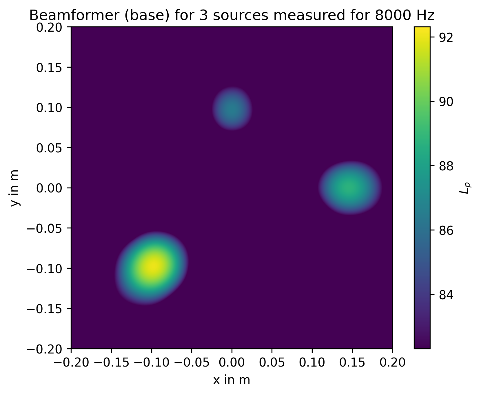
The beamforming map is plotted as:
plt.figure(1)
plt.imshow(Lm.T, origin='lower', vmin=Lm.max() - 10, extent=rg.extent, interpolation='bicubic')
plt.colorbar()
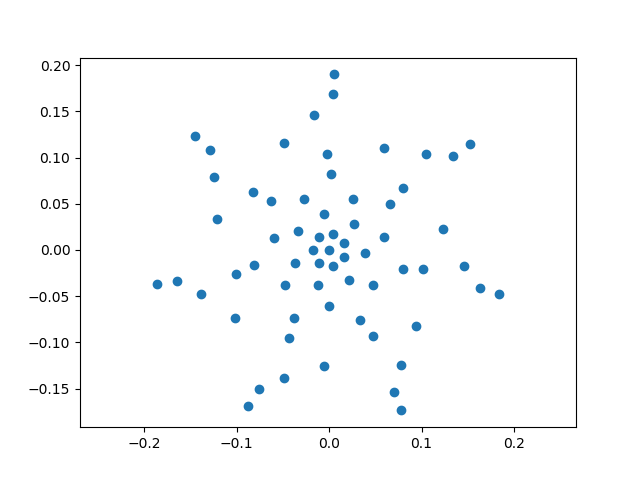
The same example also plots the microphone arrangement:
plt.figure(2)
plt.plot(mg.pos[0], mg.pos[1], 'o')
plt.axis('equal')
plt.show()
The map shows three local maxima at the simulated source positions. Their relative levels match the synthetic input data:
Source |
Location |
Level |
|---|---|---|
1 |
(-0.1,-0.1,0.3) |
1 Pa |
2 |
(0.15,0,0.3) |
0.7 Pa |
3 |
(0,0.1,0.3) |
0.5 Pa |
Next Steps#
See Lazy Evaluation for a closer look at when Acoular actually starts calculating results.
See Caching for the file-based cache controls.
Download and modify the full scripts if you want to experiment: