Note
Go to the end to download the full example code.
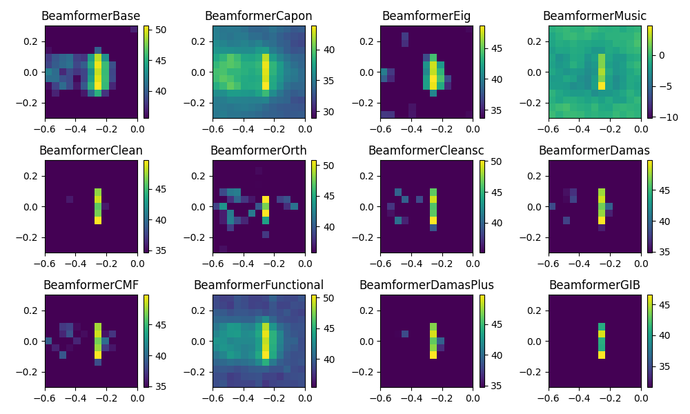
Airfoil in open jet – Frequency domain beamforming methods.#
Demonstrates different microphone array methods operating in the frequency domain. Uses measured data in file example_data.h5, calibration in file example_calib.xml, microphone geometry in array_56.xml (part of Acoular).
from pathlib import Path

import acoular as ac
from acoular.tools.helpers import get_data_file
The 4 kHz third-octave band is used for the example.
Obtain necessary data
time_data_file = get_data_file('example_data.h5')
calib_file = get_data_file('example_calib.xml')
Setting up the processing chain for the frequency domain methods.
Hint
An in-depth explanation for setting up the processing chain is given in the example Airfoil in open jet – steering vectors..
ts = ac.MaskedTimeSamples(
    file=time_data_file,
    invalid_channels=[1, 7],
    start=0,
    stop=16000,
)
calib = ac.Calib(source=ts, file=calib_file, invalid_channels=[1, 7])
mics = ac.MicGeom(file=Path(ac.__file__).parent / 'xml' / 'array_56.xml', invalid_channels=[1, 7])
grid = ac.RectGrid(x_min=-0.6, x_max=-0.0, y_min=-0.3, y_max=0.3, z=-0.68, increment=0.05)
env = ac.Environment(c=346.04)
st = ac.SteeringVector(grid=grid, mics=mics, env=env)
f = ac.PowerSpectra(source=calib, window='Hanning', overlap='50%', block_size=128)
Here, different frequency domain beamformers defined in the module fbeamform are
used and the corresponding result maps are calculated by evaluating the
synthetic() method with the desired frequency and
bandwidth.
bb = ac.BeamformerBase(freq_data=f, steer=st, r_diag=True)
bc = ac.BeamformerCapon(freq_data=f, steer=st, cached=False)
be = ac.BeamformerEig(freq_data=f, steer=st, r_diag=True, n=54)
bm = ac.BeamformerMusic(freq_data=f, steer=st, n=6)
bd = ac.BeamformerDamas(freq_data=f, steer=st, r_diag=True, n_iter=100)
bdp = ac.BeamformerDamasPlus(freq_data=f, steer=st, r_diag=True, n_iter=100)
bo = ac.BeamformerOrth(freq_data=f, steer=st, r_diag=True, eva_list=list(range(38, 54)))
bs = ac.BeamformerCleansc(freq_data=f, steer=st, r_diag=True)
bcmf = ac.BeamformerCMF(freq_data=f, steer=st, method='LassoLarsBIC')
bl = ac.BeamformerClean(freq_data=f, steer=st, r_diag=True, n_iter=100)
bf = ac.BeamformerFunctional(freq_data=f, steer=st, r_diag=False, gamma=4)
bgib = ac.BeamformerGIB(freq_data=f, steer=st, method='LassoLars', n=10)
Plot result maps for different beamformers in frequency domain
import matplotlib.pyplot as plt

plt.figure(1, (10, 6))
i1 = 1  # no of subplot
for b in (bb, bc, be, bm, bl, bo, bs, bd, bcmf, bf, bdp, bgib):
    plt.subplot(3, 4, i1)
    i1 += 1
    map = b.synthetic(cfreq, num)
    mx = ac.L_p(map.max())
    plt.imshow(ac.L_p(map.T), origin='lower', vmin=mx - 15, interpolation='nearest', extent=grid.extent)
    plt.colorbar()
    plt.title(b.__class__.__name__)
    plt.tight_layout()
plt.show()
[('example_data_cache.h5', 6)]
[('example_data_cache.h5', 7)]
[('example_data_cache.h5', 8)]
[('example_data_cache.h5', 9)]
[('example_data_cache.h5', 10)]
[('/home/runner/work/acoular/acoular/docs/source/auto_examples/cache/example_data_cache.h5', 10), ('/home/runner/work/acoular/acoular/docs/source/auto_examples/cache/psf_d5b6de07d9142e5f706e2f6841677839_cache.h5', 1)]
[('example_data_cache.h5', 11)]
[('example_data_cache.h5', 12)]
[('example_data_cache.h5', 13)]
[('/home/runner/work/acoular/acoular/docs/source/auto_examples/cache/example_data_cache.h5', 13), ('/home/runner/work/acoular/acoular/docs/source/auto_examples/cache/psf_d5b6de07d9142e5f706e2f6841677839_cache.h5', 1)]
[('example_data_cache.h5', 14)]
[('example_data_cache.h5', 15)]
[('example_data_cache.h5', 16)]
[('/home/runner/work/acoular/acoular/docs/source/auto_examples/cache/example_data_cache.h5', 16), ('/home/runner/work/acoular/acoular/docs/source/auto_examples/cache/psf_d5b6de07d9142e5f706e2f6841677839_cache.h5', 1)]
[('example_data_cache.h5', 17)]
Total running time of the script: (0 minutes 8.479 seconds)