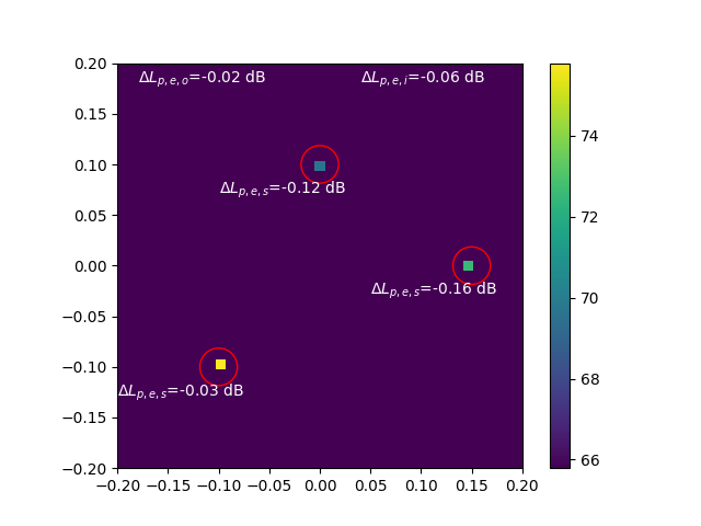
Evaluate source characterization performance.¶

This example demonstrates how to evaluate the performance of a beamforming algorithm using the acoular.tools.metrics.MetricEvaluator class to calculate the metrics introduced in [1].

from pathlib import Path

import acoular as ac
import matplotlib.pyplot as plt
import numpy as np
from acoular.tools import MetricEvaluator

Set up the parameters

sfreq = 51200
duration = 1
nsamples = duration * sfreq
micgeofile = Path(ac.__file__).parent / 'xml' / 'array_64.xml'

Generate test data, in real life this would come from an array measurement

mg = ac.MicGeom(from_file=micgeofile)
n1 = ac.WNoiseGenerator(sample_freq=sfreq, numsamples=nsamples, seed=1)
n2 = ac.WNoiseGenerator(sample_freq=sfreq, numsamples=nsamples, seed=2, rms=0.7)
n3 = ac.WNoiseGenerator(sample_freq=sfreq, numsamples=nsamples, seed=3, rms=0.5)
p1 = ac.PointSource(signal=n1, mics=mg, loc=(-0.1, -0.1, 0.3))
p2 = ac.PointSource(signal=n2, mics=mg, loc=(0.15, 0, 0.3))
p3 = ac.PointSource(signal=n3, mics=mg, loc=(0, 0.1, 0.3))
pa = ac.Mixer(source=p1, sources=[p2, p3])

Analyze the data and generate a deconvolved source map with CLEAN-SC

ps = ac.PowerSpectra(time_data=pa, block_size=128, window='Hanning')
rg = ac.RectGrid(x_min=-0.2, x_max=0.2, y_min=-0.2, y_max=0.2, z=0.3, increment=0.01)
st = ac.SteeringVector(grid=rg, mics=mg, ref=1.0)
bb = ac.BeamformerCleansc(freq_data=ps, steer=st)
pm = bb.synthetic(8000, 0)
Lm = ac.L_p(pm)

Evaluate the results: Therefore, we define a custom grid containing the source locations.

target_grid = ac.ImportGrid(
    gpos_file=np.array(
        [
            list(p1.loc),
            list(p2.loc),
            list(p3.loc),
        ],
    ).T,
)

Next, we define the target squared sound pressure values for each source.

nfft = ps.fftfreq().shape[0]
target_data = np.array([[n1.rms**2 / nfft], [n2.rms**2 / nfft], [n3.rms**2 / nfft]]).T

Finally, we use the acoular.tools.metrics.MetricEvaluator class to evaluate the reconstruction accuracy of the beamforming algorithm with three different metrics. A circular sector with a radius of 5% of the aperture is used to define the sectors for the evaluation.

mv = MetricEvaluator(
    sector=ac.CircSector(r=0.05 * mg.aperture),
    grid=rg,
    data=pm.reshape((1, -1)),
    target_grid=target_grid,
    target_data=target_data,
)

Plot the data

plt.figure()
# show map
plt.imshow(Lm.T, origin='lower', vmin=Lm.max() - 10, extent=rg.extend(), interpolation='none')
# plot sectors
ax = plt.gca()
for j, sector in enumerate(mv.sectors):
    ax.add_patch(plt.Circle((sector.x, sector.y), sector.r, color='red', fill=False))
    # annotate specific level error below circles
    plt.annotate(
        r'$\Delta L_{p,e,s}$=' + str(round(mv.get_specific_level_error()[0, j], 2)) + ' dB',
        xy=(sector.x - 0.1, sector.y - sector.r - 0.01),
        color='white',
    )
# annotate overall level error
plt.annotate(
    r'$\Delta L_{p,e,o}$=' + str(round(mv.get_overall_level_error()[0], 2)) + ' dB',
    xy=(0.05, 0.95),
    xycoords='axes fraction',
    color='white',
)
plt.annotate(
    r'$\Delta L_{p,e,i}$=' + str(round(mv.get_inverse_level_error()[0], 2)) + ' dB',
    xy=(0.6, 0.95),
    xycoords='axes fraction',
    color='white',
)
plt.colorbar()
plt.show()

Total running time of the script: (0 minutes 0.535 seconds)

Gallery generated by Sphinx-Gallery

Acoular 24.07 documentation

Evaluate source characterization performance.

Evaluate source characterization performance.¶