Note
Go to the end to download the full example code.
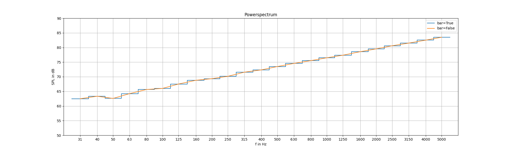
Tools – Demonstrates barspectrum tool of Acoular
A noise source emitting white noise is simulated. Its spectrum at a single microphone is plotted by using functions from acoular.tools.
import acoular as ac
import numpy as np
from acoular.tools import barspectrum

#  Set up a single microphone at (0,0,0)
m = ac.MicGeom(pos_total=np.array([[0, 0, 0]]).T)

# Create a noise source
sample_freq = 12800  # sample frequency
n1 = ac.WNoiseGenerator(sample_freq=sample_freq, num_samples=10 * sample_freq, seed=1)

t = ac.PointSource(signal=n1, mics=m, loc=(1, 0, 1))

# create power spectrum
f = ac.PowerSpectra(source=t, window='Hanning', overlap='50%', block_size=4096, cached=False)

# get spectrum data
spectrum_data = np.real(f.csm[:, 0, 0])  # get power spectrum from cross-spectral matrix
freqs = f.fftfreq()  # FFT frequencies

# use barspectrum from acoular.tools to create third octave plot data
band = 3  # octave: 1 ;   1/3-octave: 3 (for plotting)
(f_borders, p, f_center) = barspectrum(spectrum_data, freqs, band, bar=True)
(f_borders_, p_, f_center_) = barspectrum(spectrum_data, freqs, band, bar=False)
create figure with barspectra
import matplotlib.pyplot as plt

plt.figure(figsize=(20, 6))
plt.title('Powerspectrum')
plt.plot(f_borders, ac.L_p(p), label='bar=True')
plt.plot(f_borders_, ac.L_p(p_), label='bar=False')
plt.xlim(f_borders[0] * 2 ** (-1.0 / 6), f_borders[-1] * 2 ** (1.0 / 6))
plt.ylim(50, 90)
plt.xscale('symlog')
label_freqs = [str(int(_)) for _ in f_center]  # create string labels
plt.xticks(f_center, label_freqs)
plt.xlabel('f in Hz')
plt.ylabel('SPL in dB')
plt.grid(True)
plt.legend()
plt.show()
Total running time of the script: (0 minutes 0.182 seconds)